Neural Self-Organization: Growing Patterns with Neural Cellular Automata

Intro to differentiable morphogenesis and emergent self-repair

Context: Morphogenesis ≈ programmable self-assembly. A Neural Cellular Automaton (NCA) is a discrete-time, convolutional dynamical system whose transition operator is differentiable and therefore amenable to gradient-based system identification.

Scope: re-implementation of the Mordvintsev et al. (2020) NCA in PyTorch and instrument it with research-grade tooling: dynamic roll-outs, gradient clipping, Fourier/PCA diagnostics, regeneration stress-tests, and weight-space tracking.

Road-map:

Formalisation of the CA’s state-space and update equations (incl. Sobel perception)
Derivation of the training objective $\mathcal L(\theta)$ and optimisation protocol
Sample-pool curriculum and why it yields an attractor basin around the target pattern
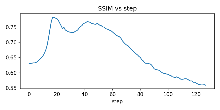
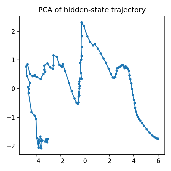
Quantitative diagnostics: SSIM/PSNR, radially-averaged power spectra, hidden-state PCA
Ablations: dropout level ↦ robustness, channel budget ↦ expressivity

Designed to run on a single GPU.

1. Foundation

Cell State Representation

Each cell $(i,j)$ maintains a 16-dimensional state vector $\mathbf{s}_{i,j}^{(t)} \in \mathbb{R}^{16}$:

RGB channels (0-2): Visual appearance $\in [0,1]$
Alpha channel (3): “Alive” marker; $\alpha > 0.1$ indicates living cell
Hidden channels (4-15): Latent variables for coordination

Update Dynamics

At each time step, cells update via:

Perception: Sobel gradient sensing: $\mathbf{p}_{i,j}^{(t)} = [\, \mathbf{s}_{i,j}^{(t)},\; \partial_x \mathbf{s}_{i,j}^{(t)},\; \partial_y \mathbf{s}_{i,j}^{(t)}\,] \in \mathbb{R}^{48}$
Neural update rule: small MLP produces increment: $\Delta \mathbf{s}_{i,j}^{(t)} = f_\theta(\mathbf{p}_{i,j}^{(t)})$
Stochastic application: asynchronous updates with probability $p=0.5$: $\mathbf{s}_{i,j}^{(t+1)} = \mathbf{s}_{i,j}^{(t)} + m_{i,j}^{(t)} \cdot \Delta \mathbf{s}_{i,j}^{(t)}$
Life/death masking: cells without living neighbors are zeroed

This creates a differentiable dynamical system where local rules can be learned via gradient descent to achieve global morphological objectives.

Formal Objective & Gradient Flow

Let $g_{\boldsymbol\theta}:\mathbb{R}^{C\times H\times W}\to\mathbb{R}^{C\times H\times W}$ denote one CA update parameterised by weights $\boldsymbol\theta$. A $T$-step rollout is the composition $g_{\boldsymbol\theta}^{\circ T}=g_{\boldsymbol\theta}\circ\cdots\circ g_{\boldsymbol\theta}$ applied $T$ times. For a distribution of initial states $\mathcal I$ (here the distribution over pool states during training) and a horizon distribution $\mathcal T$ (uniform over the schedule described later), the learning signal is the mean-squared reconstruction error between the rendered RGBA projection $\pi_{\text{rgba}}\bigl(g_{\boldsymbol\theta}^{\circ T}(\mathbf S_0)\bigr)$ and a fixed target image $\mathbf X^\star$:

\[\mathcal L(\boldsymbol\theta)\;=\; \underset{\mathbf S_0\sim\mathcal I}{\mathbb E}\; \underset{T\sim\mathcal T}{\mathbb E} \bigl\| \pi_{\text{rgba}}\!\bigl(g_{\boldsymbol\theta}^{\circ T}(\mathbf S_0)\bigr)-\mathbf X^\star \bigr\|_2^2.\]

Every operation in $g_{\boldsymbol\theta}$ (perception, the small MLP, masking, and the stochastic Bernoulli update mask) is differentiable almost everywhere (the Bernoulli mask is not differentiable w.r.t. its own random variable, gradients are conditioned on the sample and are a Monte Carlo estimate of the true expectation), the gradient $\nabla_{\boldsymbol\theta}\mathcal L$ is unbiased but stochastic gradient estimate, computed by back-propagating through the unrolled computational graph. In practice it is recommended to clip the total gradient norm to 1 to avoid exploding gradients and rely on Adam with a decayed learning rate schedule. The stochastic update mask acts as a form of spatial dropout which empirically reduces co-adaptation of neighbouring cells and encourages the emergence of truly local rules.

A useful way to interpret the CA is as a space- and time-evolving residual network. Each cell implements a residual block $\mathbf s^{(t+1)}=\mathbf s^{(t)}+\Delta\mathbf s^{(t)}$ and the alive-mask pooling enforces a soft domain constraint that prunes isolated activations, akin to morphological erosion in mathematical morphology.

2. Implementation Setup

import pathlib
import time
import json
import random
import io
import urllib.request
from typing import List
from dataclasses import dataclass, asdict

import numpy as np
import matplotlib.pyplot as plt
import seaborn as sns
import PIL.Image

import torch
import torch.nn as nn
import torch.nn.functional as F
from skimage.metrics import structural_similarity as ssim, peak_signal_noise_ratio as psnr
from sklearn.decomposition import PCA
from scipy.fft import fft2, fftshift
import imageio.v2 as imageio


torch.manual_seed(42)
np.random.seed(42)
random.seed(42)

device = torch.device("cuda" if torch.cuda.is_available() else "cpu")
if torch.backends.mps.is_available():
    device = torch.device("mps")
print(f"Running on: {device}")

FIG_DIR = pathlib.Path("figures")
FIG_DIR.mkdir(parents=True, exist_ok=True)

3. Target Pattern & Data Preparation

The implementation will train the NCA to grow a 🐣 emoji from a single seed cell.

GRID_SIZE = 64
TARGET_PATH = pathlib.Path("target.png")

if not TARGET_PATH.exists():
    print("Downloading target emoji...")
    url = "https://raw.githubusercontent.com/googlefonts/noto-emoji/main/png/128/emoji_u1f423.png"
    with urllib.request.urlopen(url) as resp:
        PIL.Image.open(io.BytesIO(resp.read())).save(TARGET_PATH)


target_img = PIL.Image.open(TARGET_PATH).convert("RGBA")
canvas = PIL.Image.new("RGBA", (GRID_SIZE, GRID_SIZE))
resized = target_img.resize((40, 40), resample=PIL.Image.BILINEAR)
canvas.paste(resized, ((GRID_SIZE - 40) // 2,) * 2, resized)

target_rgba = np.array(canvas).astype(np.float32) / 255.0
TARGET_TENSOR = torch.from_numpy(target_rgba).permute(2,0,1).unsqueeze(0).to(device)

plt.figure(figsize=(3, 3))
plt.imshow(target_rgba)
plt.axis("off")
plt.title("Target Pattern (🐣)")
plt.tight_layout()
plt.savefig(f"{FIG_DIR}/target.png", dpi=150, bbox_inches="tight")
plt.show()

4. Neural Cellular Automaton Model

The core of our system is a small convolutional network that acts as the local update rule.

class NeuralCA(nn.Module):
    """Neural Cellular Automaton with Sobel perception and residual updates."""
    def __init__(self, channels: int = 16, hidden: int = 128, dropout_p: float = 0.5):
        super().__init__()
        self.channels = channels
        self.dropout_p = dropout_p
        
        sobel_x = torch.tensor([[-1.0, 0.0, 1.0], [-2.0, 0.0, 2.0], [-1.0, 0.0, 1.0]])
        sobel_y = sobel_x.t()
        kx = sobel_x.view(1, 1, 3, 3).repeat(channels, 1, 1, 1)
        ky = sobel_y.view(1, 1, 3, 3).repeat(channels, 1, 1, 1)
        
        self.perception = nn.Conv2d(channels, 2 * channels, 3, padding=1, groups=channels, bias=False)
        self.perception.weight.data.copy_(torch.cat([kx, ky], 0))
        self.perception.weight.requires_grad_(False)
        
        self.update_net = nn.Sequential(
            nn.Conv2d(3 * channels, hidden, 1),
            nn.ReLU(),
            nn.Conv2d(hidden, channels, 1)
        )
        
        nn.init.zeros_(self.update_net[-1].weight)
        nn.init.zeros_(self.update_net[-1].bias)
    
    def alive_mask(self, x: torch.Tensor) -> torch.Tensor:
        """Compute mask of cells that should remain alive."""
        alpha = x[:, 3:4]
        neighborhood_alive = F.max_pool2d(alpha, 3, stride=1, padding=1)
        return (neighborhood_alive > 0.1).float()
    
    def forward(self, x: torch.Tensor, training: bool = True) -> torch.Tensor:
        gradients = self.perception(x)
        perception = torch.cat([x, gradients], dim=1)
        delta = self.update_net(perception)
        
        if training:
            mask = (torch.rand_like(delta[:, :1]) < (1.0 - self.dropout_p)).float()
            delta = delta * mask
        
        x = x + delta
        x = x * self.alive_mask(x)
        x[:, :4] = torch.clamp(x[:, :4], 0.0, 1.0)
        return x


def seed_state(channels: int = 16, batch: int = 1) -> torch.Tensor:
    """Create initial state with single alive cell at center."""
    state = torch.zeros(batch, channels, GRID_SIZE, GRID_SIZE, device=device)
    center = GRID_SIZE // 2
    state[:, 3:, center, center] = 1.0
    return state


def to_rgba(state_tensor: torch.Tensor) -> np.ndarray:
    """Convert state tensor to RGBA image."""
    rgba = state_tensor[0, :4].detach().cpu().numpy()
    rgba = np.moveaxis(np.clip(rgba, 0, 1), 0, -1)
    return rgba


model = NeuralCA().to(device)
test_state = seed_state()

print(f"Model parameters: {sum(p.numel() for p in model.parameters()):,}")
print(f"Seed state shape: {test_state.shape}")

plt.figure(figsize=(3, 3))
plt.imshow(to_rgba(test_state))
plt.axis("off")
plt.title("Initial Seed State")
plt.tight_layout()
plt.savefig(f"{FIG_DIR}/seed.png", dpi=150, bbox_inches="tight")
plt.show()

5. Training Strategy: The Sample Pool Method

Traditional RNN training on long sequences is memory-intensive. Instead, let’s use a “sample pool” approach:

Maintain a pool of 256 CA states at various stages of development
Each training step: sample a batch, evolve for 8-128 steps, compute loss
Replace worst-performing sample with fresh seed to maintain diversity
This implicitly trains the pattern to be a stable attractor

Why does the pool help? Without it, back-propagation would always start from the same point on the trajectory (typically the pristine seed) making the optimisation highly myopic and leading to attractors that only look correct at a single time stamp. The pool therefore acts as a replay buffer $\mathcal D={\mathbf S^{(k)}}_{k=1}^{N}$ that continually covers a diverse orbit of the current policy $g_{\boldsymbol\theta}$. Sampling from $\mathcal D$ yields the Monte Carlo estimator

\[\hat{\mathcal L}(\boldsymbol\theta)=\frac{1}{B}\sum_{b=1}^{B} \bigl\| \pi_{\text{rgba}}\!\bigl(g_{\boldsymbol\theta}^{\circ T_b}(\mathbf S_b)\bigr)-\mathbf X^\star \bigr\|_2^2,\qquad (\mathbf S_b,T_b)\sim\mathrm{Uniform}(\mathcal D)\times\mathcal T,\]

where $B=16$ in our experiments. After every gradient step we refresh the worst performer (identified by the highest loss) with a clean seed. This simple heuristic prevents the buffer from collapsing to trivial or dead states and provides an ever-present exploration pressure.

From a control-theoretic perspective the optimisation shapes $g_{\boldsymbol\theta}$ such that the target image becomes an asymptotically stable fixed point. Small perturbations (Section 7) are equivalent to bounded disturbances, and the observed convergence empirically demonstrates that the learned CA implements a robust attractor basin around $\mathbf X^\star$.

@dataclass
class TrainingConfig:
    """Configuration for NCA training experiment."""
    channels: int = 16
    hidden: int = 128
    dropout_p: float = 0.5
    lr: float = 1e-3
    pool_size: int = 256
    batch_size: int = 16
    steps: int = 8000
    rollout_start: int = 8
    rollout_growth: int = 16
    rollout_cap: int = 128
    growth_frequency: int = 2000

    def rollout_length(self, iteration: int) -> int:
        """Progressive rollout schedule: start short, grow longer for stability."""
        return min(
            self.rollout_cap,
            self.rollout_start + (iteration // self.growth_frequency) * self.rollout_growth
        )


def train_nca(config: TrainingConfig, save_artifacts: bool = True) -> dict:
    """Train Neural CA with comprehensive diagnostics."""
    
    model = NeuralCA(config.channels, config.hidden, config.dropout_p).to(device)
    optimizer = torch.optim.Adam(model.parameters(), lr=config.lr)
    scheduler = torch.optim.lr_scheduler.MultiStepLR(
        optimizer, [int(config.steps * 0.4), int(config.steps * 0.7)], gamma=0.3
    )
    
    pool = [seed_state(config.channels) for _ in range(config.pool_size)]
    
    loss_history = []
    grad_history = []
    alive_history = []
    channel_variance_history = []
    weight_snapshots = {}
    
    print(f"Training for {config.steps} iterations...")
    start_time = time.time()
    
    for iteration in range(config.steps):
        indices = np.random.choice(config.pool_size, config.batch_size, replace=False)
        batch = torch.cat([pool[i] for i in indices], dim=0)
        
        rollout_steps = np.random.randint(
            config.rollout_length(iteration) // 2,
            config.rollout_length(iteration) + 1
        )
        
        model.train()
        state = batch
        for _ in range(rollout_steps):
            state = model(state, training=True)
        
        loss = F.mse_loss(state[:, :4], TARGET_TENSOR.expand_as(state[:, :4]))
        
        optimizer.zero_grad()
        loss.backward()
        grad_norm = torch.nn.utils.clip_grad_norm_(model.parameters(), max_norm=1.0)
        optimizer.step()
        scheduler.step()
        
        for i, pool_idx in enumerate(indices):
            pool[pool_idx] = state[i:i+1].detach()
        
        worst_idx = indices[torch.argmax(loss.detach())]
        pool[worst_idx] = seed_state(config.channels)
        
        loss_history.append(loss.item())
        grad_history.append(grad_norm.item())
        alive_count = (state[:, 3] > 0.1).float().sum().item()
        alive_history.append(alive_count)
        
        if iteration % 1000 == 0:
            channel_var = state.var(dim=[0, 2, 3]).detach().cpu().numpy()
            channel_variance_history.append(channel_var)

        progress = iteration / config.steps
        if any(abs(progress - p) < 1e-3 for p in [0.0, 0.4, 0.7]) or iteration == config.steps - 1:
            weights = torch.cat([p.detach().flatten() for p in model.parameters()]).cpu().numpy()
            weight_snapshots[int(progress * 100)] = weights
        
        if (iteration + 1) % 1000 == 0:
            elapsed = time.time() - start_time
            print(f"Step {iteration + 1:5d}/{config.steps} | "
                  f"Loss: {loss.item():.4f} | "
                  f"Grad: {grad_norm:.3f} | "
                  f"Rollout: {rollout_steps:2d} | "
                  f"Time: {elapsed:.1f}s")
    
    total_time = time.time() - start_time
    print(f"Training completed in {total_time:.1f}s")
    
    results = {
        "model": model,
        "loss_history": np.array(loss_history),
        "grad_history": np.array(grad_history),
        "alive_history": np.array(alive_history),
        "channel_variance_history": np.array(channel_variance_history),
        "weight_snapshots": weight_snapshots,
        "config": config
    }
    
    if save_artifacts:
        np.savez(
            FIG_DIR / "training_metrics.npz",
            loss=results["loss_history"],
            grad_norm=results["grad_history"],
            alive_cells=results["alive_history"]
        )
        
        fig, axes = plt.subplots(1, 3, figsize=(15, 4))
        
        axes[0].semilogy(results["loss_history"])
        axes[0].set_title("Training Loss")
        axes[0].set_xlabel("Iteration")
        axes[0].set_ylabel("MSE Loss")
        
        axes[1].semilogy(results["grad_history"])
        axes[1].set_title("Gradient Norm")
        axes[1].set_xlabel("Iteration")
        axes[1].set_ylabel("L2 Norm")
        
        axes[2].plot(results["alive_history"])
        axes[2].set_title("Alive Cells")
        axes[2].set_xlabel("Iteration")
        axes[2].set_ylabel("Count")
        
        plt.tight_layout()
        plt.savefig(f"{FIG_DIR}/training_curves.png", dpi=150)
        plt.show()
    
    return results

config = TrainingConfig(steps=8000)
results = train_nca(config)
trained_model = results["model"]

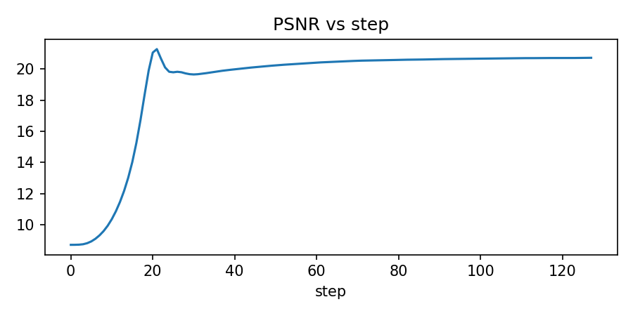
6. Growth Dynamics Analysis

Let’s analyze how the pattern develops from seed to target over time.

def analyze_growth_dynamics(model: nn.Module, steps: int = 128, save_gif: bool = True) -> tuple:
    """Analyze and visualize growth dynamics."""
    
    model.eval()
    states = []
    metrics = {"ssim": [], "psnr": [], "alive_cells": []}
    
    state = seed_state()
    target_np = TARGET_TENSOR[0].permute(1, 2, 0).cpu().numpy()
    
    with torch.no_grad():
        for step in range(steps):
            state = model(state, training=False)
            states.append(state.clone())
            
            current_img = torch.clamp(state[0, :4], 0, 1).permute(1, 2, 0).cpu().numpy()
            metrics["ssim"].append(ssim(current_img, target_np, channel_axis=2, data_range=1.0))
            metrics["psnr"].append(psnr(target_np, current_img, data_range=1.0))
            metrics["alive_cells"].append((state[0, 3] > 0.1).float().sum().item())
    
    n_frames = 16
    frame_indices = np.linspace(0, len(states)-1, n_frames).astype(int)
    
    fig, axes = plt.subplots(2, 8, figsize=(16, 4))
    axes = axes.flatten()
    
    for i, idx in enumerate(frame_indices):
        axes[i].imshow(to_rgba(states[idx]))
        axes[i].axis("off")
        axes[i].set_title(f"Step {idx}")
    
    plt.suptitle("Growth Progression", fontsize=16)
    plt.tight_layout()
    plt.savefig(f"{FIG_DIR}/growth_montage.png", dpi=150, bbox_inches="tight")
    plt.show()
    
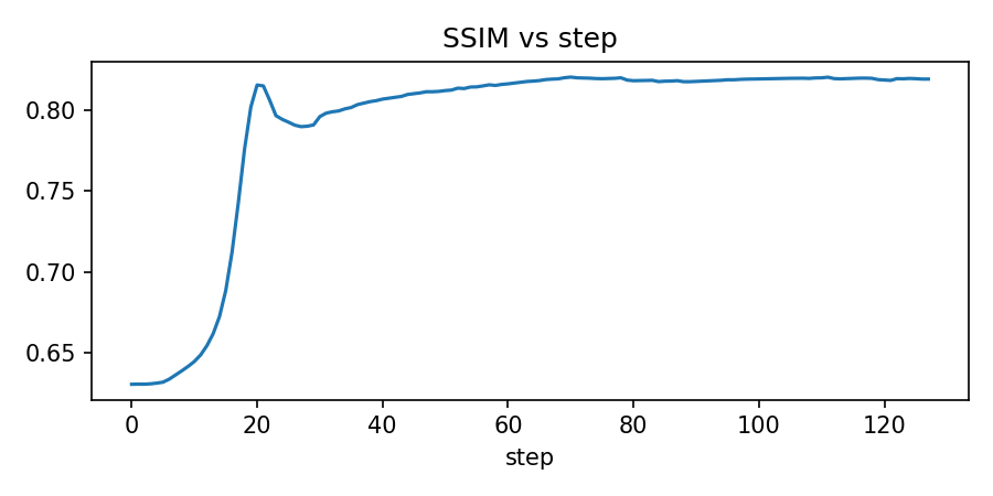
    fig, axes = plt.subplots(1, 3, figsize=(15, 4))
    
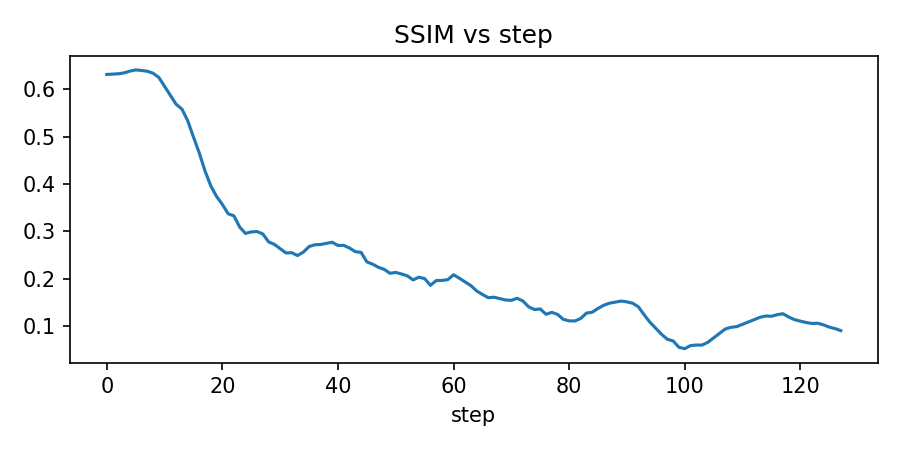
    axes[0].plot(metrics["ssim"])
    axes[0].set_title("Structural Similarity (SSIM)")
    axes[0].set_xlabel("Step")
    axes[0].set_ylabel("SSIM")
    axes[0].grid(True, alpha=0.3)
    
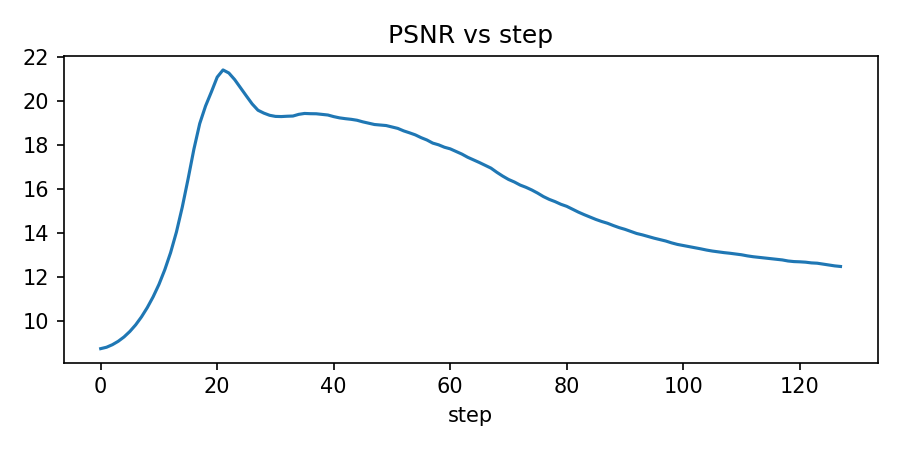
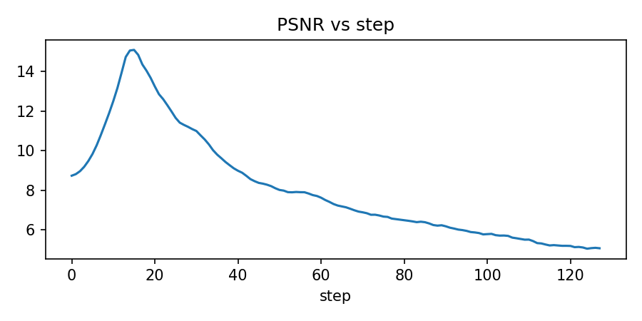
    axes[1].plot(metrics["psnr"])
    axes[1].set_title("Peak Signal-to-Noise Ratio")
    axes[1].set_xlabel("Step")
    axes[1].set_ylabel("PSNR (dB)")
    axes[1].grid(True, alpha=0.3)
    
    axes[2].plot(metrics["alive_cells"])
    axes[2].set_title("Living Cell Count")
    axes[2].set_xlabel("Step")
    axes[2].set_ylabel("Cells")
    axes[2].grid(True, alpha=0.3)
    
    plt.tight_layout()
    plt.savefig(f"{FIG_DIR}/convergence_metrics.png", dpi=150)
    plt.show()
    
    if save_gif:
        gif_frames = []
        for i in range(0, len(states), 2):
            frame = (to_rgba(states[i]) * 255).astype(np.uint8)
            gif_frames.append(frame)
        
        imageio.mimsave(FIG_DIR / "growth_animation.gif", gif_frames, fps=8)
        print(f"Saved growth animation: {FIG_DIR / 'growth_animation.gif'}")
    
    return states, metrics


growth_states, growth_metrics = analyze_growth_dynamics(trained_model)

7. Regeneration Capability

A hallmark of biological systems is the ability to regenerate damaged tissue. Let’s test our NCA’s regenerative properties.

def test_regeneration(model: nn.Module, damage_radius: int = 12, healing_steps: int = 96) -> tuple:
    """Test the model's ability to regenerate after damage."""
    
    model.eval()
    
    state = seed_state()
    with torch.no_grad():
        for _ in range(80):
            state = model(state, training=False)
    
    pre_damage = state.clone()
    
    center = GRID_SIZE // 2
    y, x = torch.meshgrid(torch.arange(GRID_SIZE), torch.arange(GRID_SIZE), indexing="ij")
    damage_mask = ((x - center)**2 + (y - center)**2) < damage_radius**2
    state[:, :, damage_mask] = 0.0
    
    damaged = state.clone()
    
    healing_states = [state.clone()]
    with torch.no_grad():
        for _ in range(healing_steps):
            state = model(state, training=False)
            healing_states.append(state.clone())
    
    healed = state.clone()
    
    fig, axes = plt.subplots(1, 4, figsize=(16, 4))
    
    axes[0].imshow(to_rgba(pre_damage))
    axes[0].set_title("Before Damage")
    axes[0].axis("off")
    
    axes[1].imshow(to_rgba(damaged))
    axes[1].set_title(f"After Damage (r={damage_radius})")
    axes[1].axis("off")
    
    axes[2].imshow(to_rgba(healed))
    axes[2].set_title(f"After Healing ({healing_steps} steps)")
    axes[2].axis("off")
    
    diff = torch.abs(pre_damage - healed).mean(dim=1, keepdim=True)
    axes[3].imshow(diff[0, 0].cpu().numpy(), cmap="hot")
    axes[3].set_title("Recovery Difference")
    axes[3].axis("off")
    
    plt.suptitle("Regeneration Test", fontsize=16)
    plt.tight_layout()
    plt.savefig(f"{FIG_DIR}/regeneration_test.png", dpi=150, bbox_inches="tight")
    plt.show()
    
    gif_frames = []
    for state in healing_states[::2]:
        frame = (to_rgba(state) * 255).astype(np.uint8)
        gif_frames.append(frame)
    
    imageio.mimsave(FIG_DIR / "healing_animation.gif", gif_frames, fps=6)
    print(f"Saved healing animation: {FIG_DIR / 'healing_animation.gif'}")
    
    return pre_damage, damaged, healed, healing_states

pre_dmg, damaged, healed, healing_sequence = test_regeneration(trained_model)

8. NCA Dynamics Analysis

Let’s conduct deeper analysis of the learned dynamics.

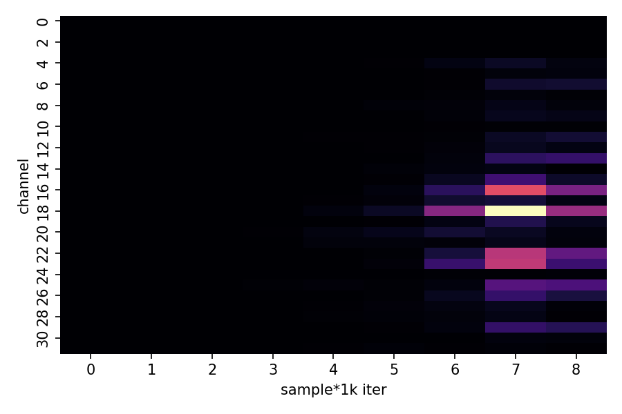
def analyze_nca_dynamics(model: nn.Module, growth_states: List[torch.Tensor], results: dict) -> None:
    """Perform analysis of NCA dynamics."""
    
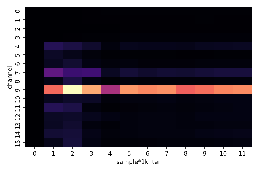
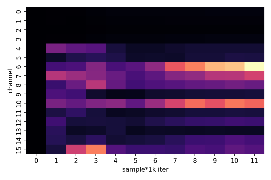
    channel_vars = np.array(results["channel_variance_history"])
    if channel_vars.size > 0:
        plt.figure(figsize=(10, 6))
        sns.heatmap(channel_vars.T, cmap="magma", cbar_kws={"label": "Variance"})
        plt.title("Channel Activity During Training")
        plt.xlabel("Training Epoch (×1000)")
        plt.ylabel("Channel Index")
        plt.tight_layout()
        plt.savefig(f"{FIG_DIR}/channel_activity.png", dpi=150)
        plt.show()
    
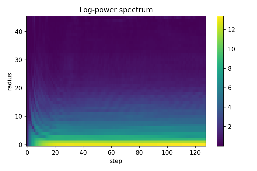
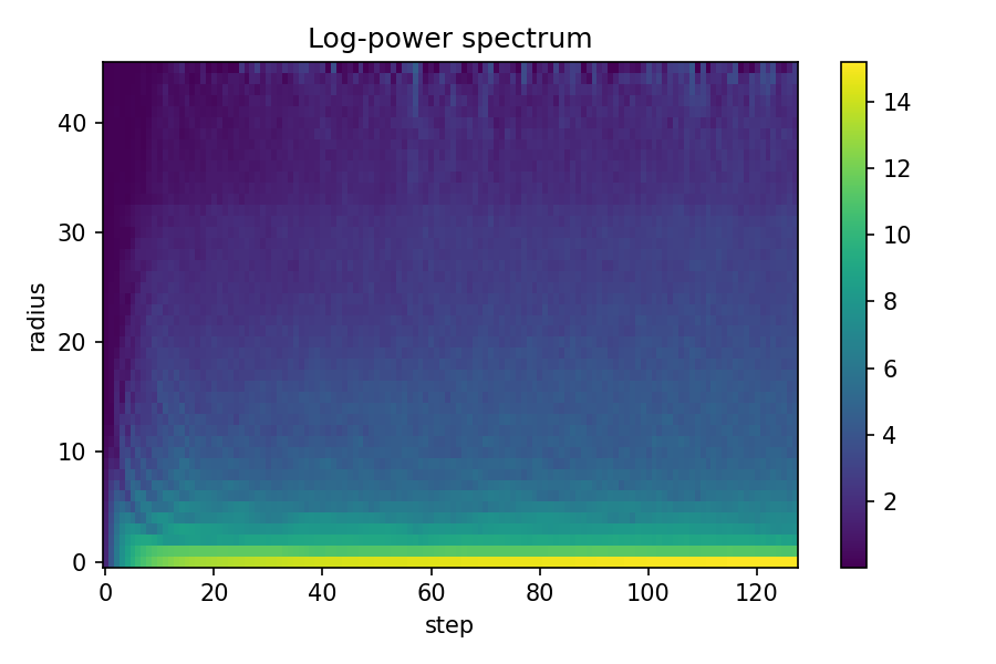
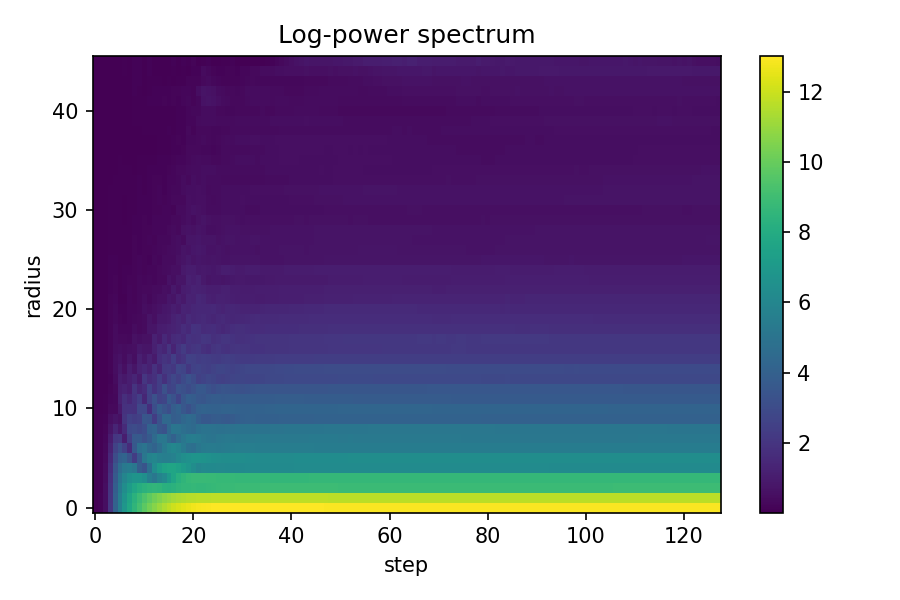
    def radial_power_spectrum(image: np.ndarray) -> np.ndarray:
        """Compute radially-averaged power spectrum."""
        gray = image.mean(0) if image.ndim == 3 else image
        F = np.abs(fftshift(fft2(gray)))**2
        
        h, w = F.shape
        y, x = np.indices((h, w))
        r = np.sqrt((x - w//2)**2 + (y - h//2)**2).astype(int)
        
        r_max = min(h, w) // 2
        power_profile = np.zeros(r_max)
        for radius in range(r_max):
            mask = (r == radius)
            if mask.any():
                power_profile[radius] = F[mask].mean()
        
        return power_profile
    
    spectra = []
    for state in growth_states[::8]:
        rgb = torch.clamp(state[0, :3], 0, 1).cpu().numpy()
        spectrum = radial_power_spectrum(rgb)
        spectra.append(spectrum)
    
    spectra_matrix = np.array(spectra)
    
    plt.figure(figsize=(10, 6))
    plt.imshow(spectra_matrix.T, aspect="auto", cmap="viridis", origin="lower")
    plt.colorbar(label="Log Power")
    plt.title("Fourier Spectrum Evolution")
    plt.xlabel("Growth Step (×8)")
    plt.ylabel("Spatial Frequency")
    plt.tight_layout()
    plt.savefig(f"{FIG_DIR}/spectrum_evolution.png", dpi=150)
    plt.show()
    
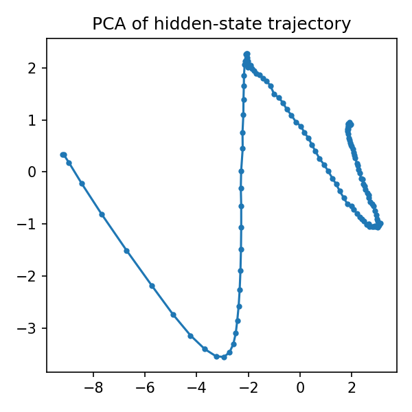
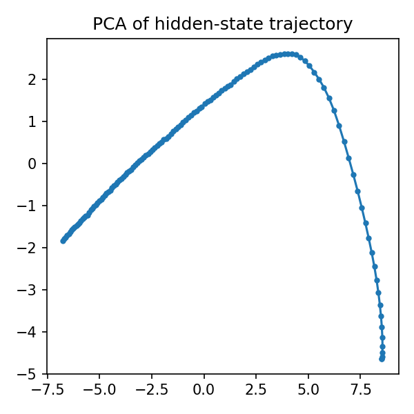
    hidden_means = []
    for state in growth_states:
        hidden = state[0, 4:].cpu().numpy()
        mean_hidden = hidden.reshape(hidden.shape[0], -1).mean(axis=1)
        hidden_means.append(mean_hidden)
    
    hidden_array = np.array(hidden_means)
    
    if hidden_array.shape[1] >= 2:
        X = hidden_array.astype(np.float64)
        X = np.nan_to_num(X, nan=0.0, posinf=0.0, neginf=0.0)
        X = (X - X.mean(0)) / (X.std(0) + 1e-6)
        X = np.clip(X, -10, 10)
        
        try:
            pca = PCA(n_components=2)
            trajectory = pca.fit_transform(X)
            
            plt.figure(figsize=(8, 6))
            plt.plot(trajectory[:, 0], trajectory[:, 1], "b-", alpha=0.7, linewidth=2)
            plt.scatter(trajectory[0, 0], trajectory[0, 1], c="green", s=100, label="Start", zorder=5)
            plt.scatter(trajectory[-1, 0], trajectory[-1, 1], c="red", s=100, label="End", zorder=5)
            plt.title("Hidden State Trajectory (PCA)")
            plt.xlabel(f"PC1 ({pca.explained_variance_ratio_[0]:.1%} variance)")
            plt.ylabel(f"PC2 ({pca.explained_variance_ratio_[1]:.1%} variance)")
            plt.legend()
            plt.grid(True, alpha=0.3)
            plt.tight_layout()
            plt.savefig(f"{FIG_DIR}/hidden_trajectory.png", dpi=150)
            plt.show()
        except Exception as e:
            print(f"PCA analysis failed: {e}")
    
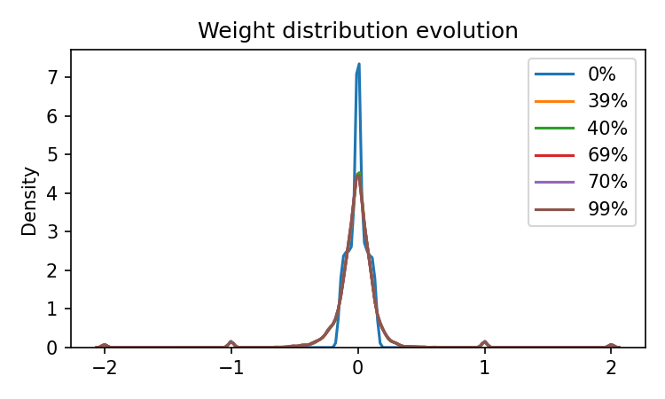
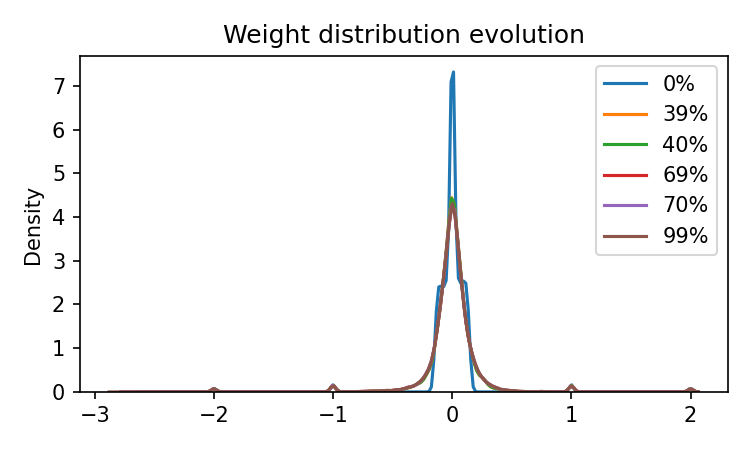
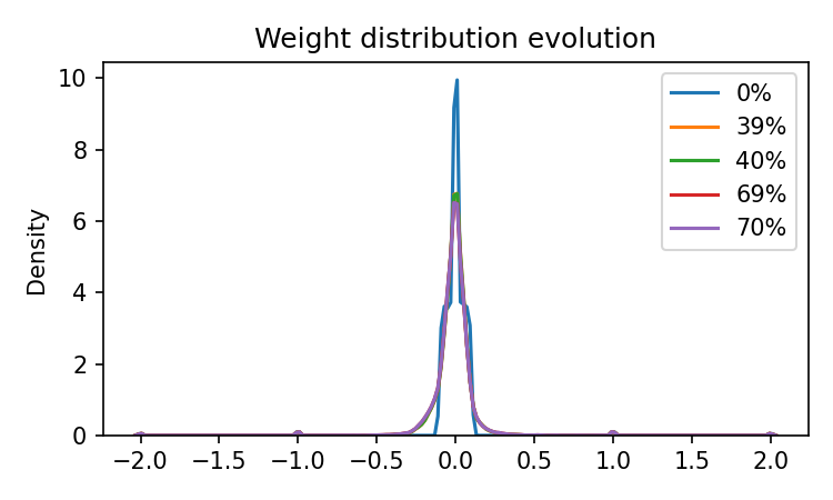
    plt.figure(figsize=(10, 6))
    for label, weights in results["weight_snapshots"].items():
        sns.kdeplot(weights, label=f"{label}% training", alpha=0.7)
    
    plt.title("Weight Distribution Evolution")
    plt.xlabel("Weight Value")
    plt.ylabel("Density")
    plt.legend()
    plt.grid(True, alpha=0.3)
    plt.tight_layout()
    plt.savefig(f"{FIG_DIR}/weight_evolution.png", dpi=150)
    plt.show()
    
    damage_radii = [4, 8, 12, 16, 20]
    recovery_times = []
    
    print("Testing recovery performance...")
    model.eval()
    target_np = TARGET_TENSOR[0].permute(1, 2, 0).cpu().numpy()
    
    for radius in damage_radii:
        state = seed_state()
        with torch.no_grad():
            for _ in range(80):
                state = model(state, training=False)
        
        center = GRID_SIZE // 2
        y, x = torch.meshgrid(torch.arange(GRID_SIZE), torch.arange(GRID_SIZE), indexing="ij")
        mask = ((x - center)**2 + (y - center)**2) < radius**2
        state[:, :, mask] = 0.0
        
        steps = 0
        max_steps = 200
        with torch.no_grad():
            while steps < max_steps:
                state = model(state, training=False)
                steps += 1
                
                current_img = torch.clamp(state[0, :4], 0, 1).permute(1, 2, 0).cpu().numpy()
                if ssim(current_img, target_np, channel_axis=2, data_range=1.0) > 0.9:
                    break
        
        recovery_times.append(steps)
        print(f"  Damage radius {radius}: {steps} steps to recover")
    
    plt.figure(figsize=(8, 6))
    plt.plot(damage_radii, recovery_times, "o-", linewidth=2, markersize=8)
    plt.title("Regeneration Performance")
    plt.xlabel("Damage Radius (pixels)")
    plt.ylabel("Steps to Recover (SSIM > 0.9)")
    plt.grid(True, alpha=0.3)
    plt.tight_layout()
    plt.savefig(f"{FIG_DIR}/recovery_performance.png", dpi=150)
    plt.show()

analyze_nca_dynamics(trained_model, growth_states, results)

9. Multiple Experimental Configurations

Let’s compare different training configurations to understand the impact of various hyperparameters.

experiments = [
    TrainingConfig(dropout_p=0.5, steps=4000),
    TrainingConfig(dropout_p=0.8, steps=4000),
    TrainingConfig(channels=32, hidden=256, steps=4000),
]

experiment_names = ["Baseline", "High Dropout", "Large Model"]
experiment_results = []

print("Running comparative experiments...")
for i, (config, name) in enumerate(zip(experiments, experiment_names)):
    print(f"\n--- Experiment {i+1}: {name} ---")
    results = train_nca(config, save_artifacts=False)
    experiment_results.append(results)

fig, axes = plt.subplots(2, 2, figsize=(12, 10))

for i, (results, name) in enumerate(zip(experiment_results, experiment_names)):
    axes[0, 0].semilogy(results["loss_history"], label=name, alpha=0.8)
axes[0, 0].set_title("Training Loss Comparison")
axes[0, 0].set_xlabel("Iteration")
axes[0, 0].set_ylabel("MSE Loss")
axes[0, 0].legend()
axes[0, 0].grid(True, alpha=0.3)

for i, (results, name) in enumerate(zip(experiment_results, experiment_names)):
    axes[0, 1].semilogy(results["grad_history"], label=name, alpha=0.8)
axes[0, 1].set_title("Gradient Norm Comparison")
axes[0, 1].set_xlabel("Iteration")
axes[0, 1].set_ylabel("L2 Norm")
axes[0, 1].legend()
axes[0, 1].grid(True, alpha=0.3)

for i, (results, name) in enumerate(zip(experiment_results, experiment_names)):
    model = results["model"]
    model.eval()
    
    state = seed_state()
    with torch.no_grad():
        for _ in range(96):
            state = model(state, training=False)
    
    axes[1, i].imshow(to_rgba(state))
    axes[1, i].set_title(f"Final Pattern: {name}")
    axes[1, i].axis("off")

if len(experiments) < 3:
    fig.delaxes(axes[1, 2])

plt.tight_layout()
plt.savefig(f"{FIG_DIR}/experiment_comparison.png", dpi=150, bbox_inches="tight")
plt.show()

10. Experiment Results

Baseline

High Dropout

Large Channels

References:

Mordvintsev, et al. “Growing Neural Cellular Automata.” Distill, 2020.